Chapter 4 Model development and evaluation
This chapter focused on model development and evaluation. Section 4.1 specified the outcomes and candidate predictors for model development. Section 4.2 introduced the three algorithms for model development and section 4.3 highlighted the procedure of evaluating model performance. Sections 4.4 and 4.5 presented the results and discussions.
4.1 Outcomes and predictors
To predict the risk of developing POI by age threshold ranging from 21 to 39, the outcomes were defined as whether a female CCS developed POI by age 21, 22, …, and 39, accordingly. The proportions of components of outcomes by the nineteen different age thresholds were listed in Table 4.1. As the age threshold increased from 21 to 39, the proportion of subjects with censored ovarian status increased significantly from 5.3% to 60.1%.
| Cut.off.age | Normal | SPM | POI | Censoring | Missing | Total |
|---|---|---|---|---|---|---|
| 21 | 6809 (86.4%) | 13 (0.2%) | 607 (7.7%) | 416 (5.3%) | 38 (0.5%) | 7883 (100%) |
| 22 | 6605 (83.8%) | 16 (0.2%) | 639 (8.1%) | 582 (7.4%) | 38 (0.5%) | 7880 (100%) |
| 23 | 6417 (81.5%) | 18 (0.2%) | 658 (8.4%) | 747 (9.5%) | 38 (0.5%) | 7878 (100%) |
| 24 | 6208 (78.8%) | 19 (0.2%) | 680 (8.6%) | 931 (11.8%) | 38 (0.5%) | 7876 (100%) |
| 25 | 5968 (75.8%) | 23 (0.3%) | 703 (8.9%) | 1140 (14.5%) | 38 (0.5%) | 7872 (100%) |
| 26 | 5707 (72.6%) | 28 (0.4%) | 718 (9.1%) | 1374 (17.5%) | 38 (0.5%) | 7865 (100%) |
| 27 | 5475 (69.7%) | 40 (0.5%) | 727 (9.3%) | 1575 (20.1%) | 38 (0.5%) | 7855 (100%) |
| 28 | 5201 (66.3%) | 47 (0.6%) | 736 (9.4%) | 1824 (23.2%) | 38 (0.5%) | 7846 (100%) |
| 29 | 4925 (62.8%) | 60 (0.8%) | 748 (9.5%) | 2072 (26.4%) | 38 (0.5%) | 7843 (100%) |
| 30 | 4617 (58.9%) | 72 (0.9%) | 756 (9.7%) | 2350 (30%) | 38 (0.5%) | 7833 (100%) |
| 31 | 4296 (54.9%) | 91 (1.2%) | 782 (10%) | 2619 (33.5%) | 38 (0.5%) | 7826 (100%) |
| 32 | 3987 (51%) | 111 (1.4%) | 793 (10.1%) | 2891 (37%) | 38 (0.5%) | 7820 (100%) |
| 33 | 3667 (46.9%) | 135 (1.7%) | 813 (10.4%) | 3162 (40.5%) | 38 (0.5%) | 7815 (100%) |
| 34 | 3372 (43.2%) | 148 (1.9%) | 829 (10.6%) | 3422 (43.8%) | 38 (0.5%) | 7809 (100%) |
| 35 | 3034 (38.9%) | 173 (2.2%) | 841 (10.8%) | 3716 (47.6%) | 38 (0.5%) | 7802 (100%) |
| 36 | 2715 (34.9%) | 197 (2.5%) | 864 (11.1%) | 3975 (51%) | 38 (0.5%) | 7789 (100%) |
| 37 | 2424 (31.1%) | 220 (2.8%) | 878 (11.3%) | 4223 (54.3%) | 38 (0.5%) | 7783 (100%) |
| 38 | 2127 (27.4%) | 234 (3%) | 888 (11.4%) | 4488 (57.7%) | 38 (0.5%) | 7775 (100%) |
| 39 | 1894 (24.4%) | 258 (3.3%) | 905 (11.7%) | 4668 (60.1%) | 38 (0.5%) | 7763 (100%) |
| 40 | 1682 (21.7%) | 273 (3.5%) | 917 (11.8%) | 4852 (62.5%) | 38 (0.5%) | 7762 (100%) |
The candidate predictors included race, cancer diagnosis type, age at diagnosis, radiation dose, chemotherapy agents, and BMT. Race and cancer diagnosis type were categorical variables. For the ten alkylating agents and their derived cumulative dose CED, the information would be redundant if included all of them in one model. Therefore, two sets of variables were prepared separately; each of them considered either ten individual alkylating agents or CED. A summary of the candidate predictors was listed in Table 4.2.
| Type of variables | Candidate predictors setting 1 | Candidate predictors setting 2 |
|---|---|---|
| Categorical | Race (3 levels) white(reference), black, and other diagnosis (8 levels) leukemia(reference), central nervous system cancers, neuroblastoma, non-Hodgkin lymphoma, Hodgkin lymphoma, kidney cancer, bone tumors, soft-tissue sarcoma BMT (Yes/No) |
Race (3 levels) white(reference), black, and other diagnosis (8 levels) leukemia(reference), central nervous system cancers, neuroblastoma, non-Hodgkin lymphoma, Hodgkin lymphoma, kidney cancer, bone tumors, soft-tissue sarcoma BMT (Yes/No) |
| Continuous: Irradiation dose (Gy) | total body irradiation dose, minmum ovary radiation dose, radiation dose to pituitary |
total body irradiation dose, minmum ovary radiation dose, radiation dose to pituitary |
| Continuous: Alkylating agents’ doses (g/m2) |
CED | BCNU, Busulfan, CCNU, Chlorambucil, Cyclophosphamide, Ifosfamide, Melphalan, Nitrogen Mustard, Procarbazine, Thiotepa |
| Continuous: Other chemotherapy agents’ doses (g/m2) |
Carboplatin, Cis_Platinum Bleomycin Daunorubicin Doxorubicin Epirubicin Idarubicin Methotrexate Mitoxantrone VM 26 VP 16 |
Carboplatin, Cis_Platinum Bleomycin Daunorubicin Doxorubicin Epirubicin Idarubicin Methotrexate Mitoxantrone VM 26 VP 16 |
4.2 Algorithms for model development
Two machine learning algorithms: Elastic-Net panelized age-specific logistic regression (EN-ALR) (Zou and Hastie 2005b) and XGBoost (T. Chen and Guestrin 2016a) were used to mapping predictors to outcomes (details about the algorithms were available in Appendix G). The third algorithm “Ensemble” averaged the predicted risks from the previous two.
The candidate predictors (Table G.1 in Appendix G) in EN-ALR and XGBoost were the same except for some rarely used chemotherapy agents (i.e. busulfan, CCNU, chlorambucil, melphalan, thiotepa, idarubicin, and mitoxantrone). These chemotherapy agents were coded as binary Yes/No in EN-ALR but were retained as continuous variables in XGBoost as the algorithm automatically choose the split-point to maximize the information gain.
Both EN-ALR and XGBoost select predictors automatically through tuning hyperparameters. As a result, once the hyperparameters are selected, the model is fixed accordingly. Therefore, tuning hyperparameters is a key step that decides the performance of the final model. In this study, I employed the “random search” (Bergstra and Bengio, n.d.) approach to tune hyperparameters in a prespecified hyperparameter space (Appendix G).
4.3 Procedures for model evaluation
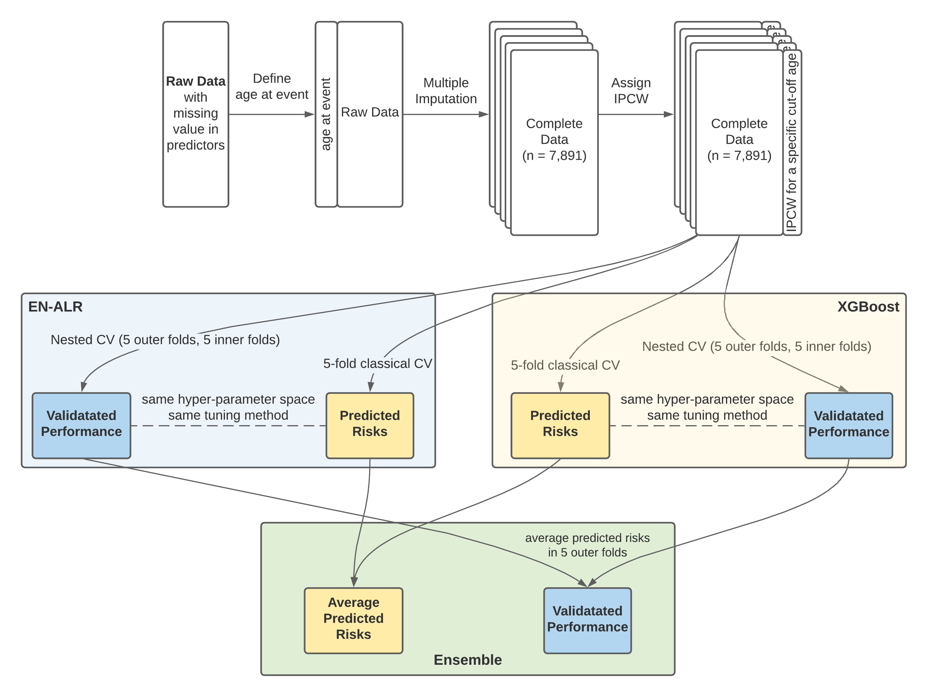
Typically, model evaluation and hyperparameter tunning are conducted in the same CV process. However, this evaluation procedure may be overoptimistic about the model performance because the hyperparameters tuned in the training set were chosen based on the model performance in validation sets. To address this issue, I employed a nested CV to evaluate the performance of the modeling procedure. The rationality of nested CV was that it constructed two layers of CV: the inner CV was used for tunning hyperparameters and the outer CV was served for evaluating model performance (Appendix E).
In summary, I used a classical CV to obtain the optimal hyperparameters and a nested CV to evaluate the performance of the modeling procedure (rather than the final model). The whole modeling process was illustrated in a schematic diagram (Figure 4.1).

Figure 4.1: Variable importance in the random survival forest model for censoring
It should be noted that combining MI and nested CV generated 125 different data sets (see Chapter 3.1.3); therefore, for each hyperparameter setting, there were 125 models developed to predict the risk of POI, and the average of the 125 predicted risks on one subject was used as her final predicted risk.
The performance matrices used in this research include areas under the receiver operating characteristic curves (AUC) and average positive predictive value (AP) for measuring the ability of discriminatory and prospective prediction. Scaled Brier Score (sBrS) was used to describe the overall model performance.
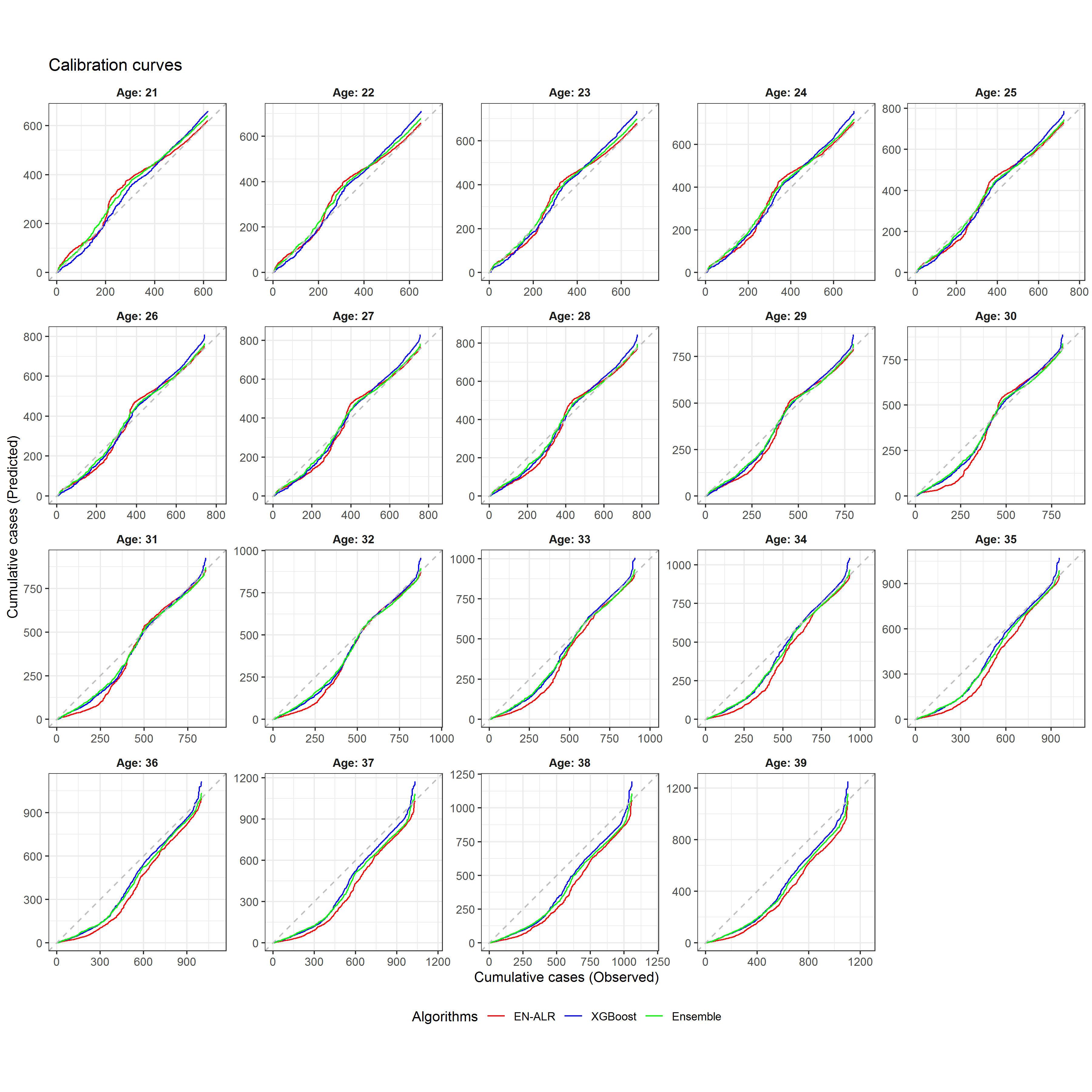
In addition, calibration curves that compared cumulative weighted predicted risk and cumulative weighted events were used to visually inspect the calibration of models.
4.4 Results
The results from nested CV showed that the performance of models with ten individual alkylating agents was superior to the models with CED (Appendix H). Therefore, the models with ten individual alkylating agents will be used and presented in the remaining sections in this chapter.
4.4.1 Predictors
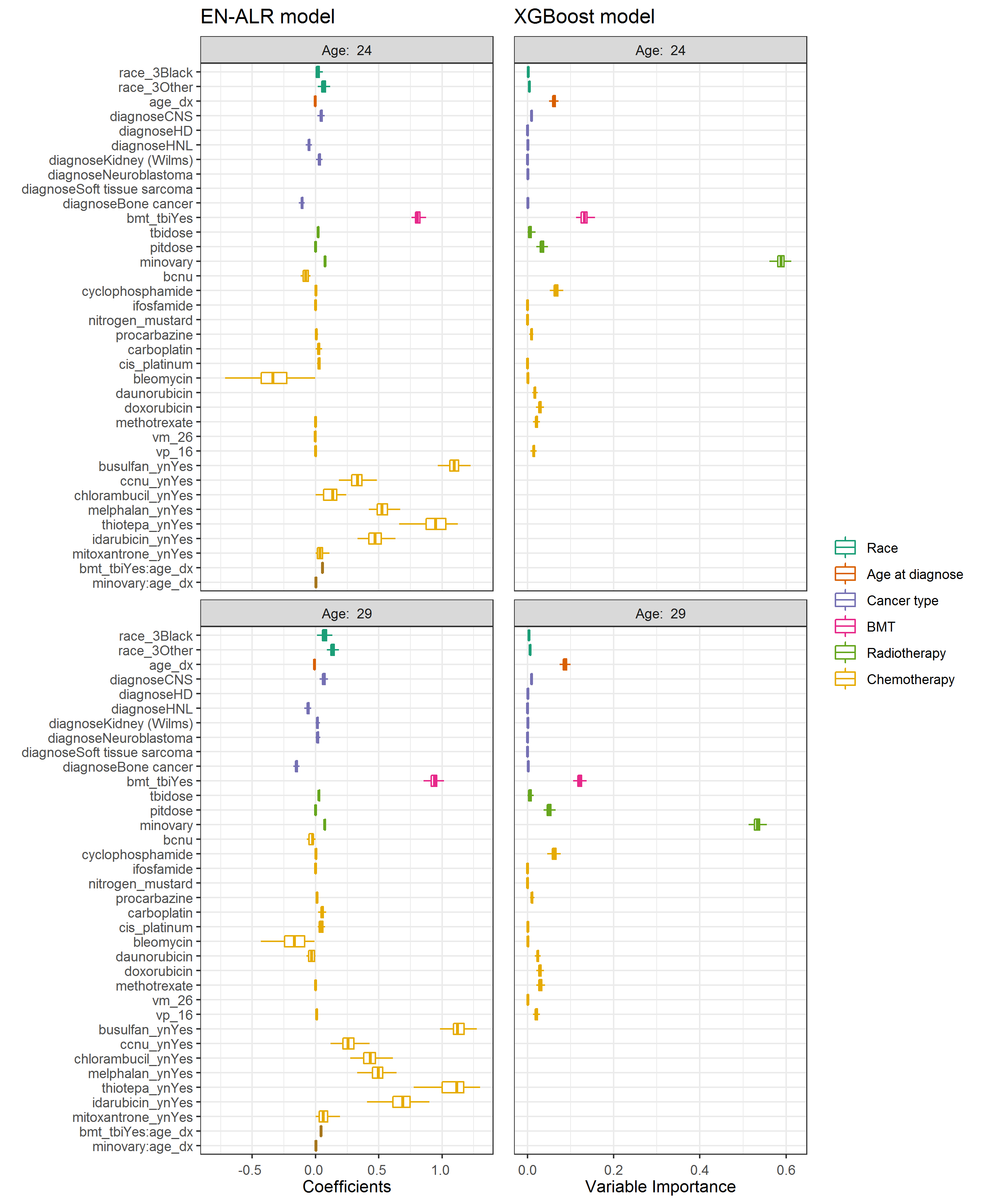
Figure 4.2 illustrated the predictors selected by EN-ALR and XGBoost when the age threshold was 24 and 29, respectively. The boxplots in the left panel showed the coefficients of each variable in the 125 EN-ALR models and the boxplots in the right panel showed the variable importance in the 125 XGBoost models. If a variable was not selected by any of the 125 models, the corresponding boxplot was absent. For example, rarely used chemotherapy agents such as busulfan, CCNU, chlorambucil, melphalan, thiotepa, idarubicin, and mitoxantrone were not selected by XGBoost. Therefore, no boxplots were available for these predictors in the right panel. The width of a boxplot reflected the variation in coefficients or variable importance of the corresponding predictor across the 125 data sets.

Figure 4.2: Predictors in the two algorithms. Left: coefficients in EN-ALR; Right: variable importance in XGBoost
The frequencies of the predictors selected by the 125 models as well as their range of values were shown in Table 4.3 and Table 4.4 for ages 24 and 29, respectively. For better visualization of the coefficients of radiotherapy and chemotherapy, the unit of irradiation doses was set to be Gy, and the unit of chemotherapy agent doses was set to be \(g/m^2\).
| Variables | EN-ALR Proportions (%) | EN-ALR Median [min, max] | XGBoost Proportions (%) | XGBoost Median [min, max] |
|---|---|---|---|---|
| race_3Black | 0.616 | 0.016 [0.001,0.077] | 0.640 | 0.002 [0,0.004] |
| race_3Other | 1.000 | 0.063 [0.018,0.123] | 1.000 | 0.004 [0.003,0.007] |
| age_dx | 1.000 | -0.004 [-0.004,-0.002] | 1.000 | 0.061 [0.047,0.079] |
| diagnoseCNS | 0.992 | 0.046 [0.005,0.072] | 1.000 | 0.009 [0.007,0.014] |
| diagnoseHNL | 1.000 | -0.052 [-0.08,-0.028] | 0.088 | 0.001 [0.001,0.001] |
| diagnoseKidney (Wilms) | 0.968 | 0.033 [0.004,0.068] | 0.560 | 0.001 [0,0.003] |
| diagnoseBone cancer | 1.000 | -0.107 [-0.141,-0.087] | 0.728 | 0.001 [0,0.002] |
| bmt_tbiYes | 1.000 | 0.806 [0.729,0.874] | 1.000 | 0.133 [0.113,0.17] |
| tbidose | 1.000 | 0.021 [0.008,0.033] | 0.864 | 0.004 [0,0.031] |
| pitdose | 0.008 | 0 [0,0] | 1.000 | 0.033 [0.02,0.052] |
| minovary | 1.000 | 0.075 [0.069,0.079] | 1.000 | 0.588 [0.561,0.618] |
| bcnu | 0.016 | -0.078 [-0.118,-0.039] | NA | NA |
| cyclophosphamide | 0.992 | 0.003 [0,0.008] | 1.000 | 0.066 [0.052,0.087] |
| ifosfamide | 0.024 | 0 [0,0] | 0.344 | 0 [0,0.001] |
| procarbazine | 0.896 | 0.006 [0,0.02] | 1.000 | 0.009 [0.003,0.015] |
| carboplatin | 0.944 | 0.024 [0,0.064] | NA | NA |
| cis_platinum | 0.016 | 0.027 [0.013,0.041] | 0.112 | 0 [0,0.002] |
| bleomycin | 0.944 | -0.338 [-0.805,-0.002] | 0.928 | 0.001 [0,0.005] |
| methotrexate | 0.992 | 0 [-0.001,0] | 1.000 | 0.022 [0.013,0.035] |
| vm_26 | 0.056 | -0.001 [-0.006,0] | NA | NA |
| vp_16 | 0.056 | 0.001 [0,0.006] | 1.000 | 0.015 [0.007,0.024] |
| busulfan_ynYes | 1.000 | 1.097 [0.945,1.225] | NA | NA |
| ccnu_ynYes | 1.000 | 0.331 [0.117,0.484] | NA | NA |
| chlorambucil_ynYes | 0.232 | 0.136 [0,0.242] | NA | NA |
| melphalan_ynYes | 1.000 | 0.525 [0.422,0.707] | NA | NA |
| thiotepa_ynYes | 1.000 | 0.949 [0.66,1.125] | NA | NA |
| idarubicin_ynYes | 1.000 | 0.472 [0.238,0.696] | NA | NA |
| mitoxantrone_ynYes | 0.264 | 0.034 [0.001,0.183] | NA | NA |
| bmt_tbiYes:age_dx | 1.000 | 0.055 [0.048,0.06] | NA | NA |
| minovary:age_dx | 1.000 | 0.002 [0.002,0.003] | NA | NA |
| diagnoseHD | NA | NA | 0.416 | 0 [0,0.003] |
| diagnoseNeuroblastoma | NA | NA | 0.848 | 0.001 [0,0.003] |
| nitrogen_mustard | NA | NA | 0.008 | 0 [0,0] |
| daunorubicin | NA | NA | 1.000 | 0.017 [0.011,0.023] |
| doxorubicin | NA | NA | 1.000 | 0.029 [0.02,0.04] |
| Variables | EN-ALR Proportions (%) | EN-ALR Median [min, max] | XGBoost Proportions (%) | XGBoost Median [min, max] |
|---|---|---|---|---|
| race_3Black | 1.000 | 0.072 [0.012,0.144] | 1.000 | 0.003 [0,0.006] |
| race_3Other | 1.000 | 0.135 [0.082,0.188] | 1.000 | 0.006 [0.004,0.009] |
| age_dx | 1.000 | -0.009 [-0.01,-0.007] | 1.000 | 0.086 [0.069,0.104] |
| diagnoseCNS | 1.000 | 0.065 [0.012,0.098] | 1.000 | 0.009 [0.006,0.012] |
| diagnoseHNL | 1.000 | -0.06 [-0.1,-0.033] | 0.512 | 0 [0,0.002] |
| diagnoseKidney (Wilms) | 0.664 | 0.015 [0.001,0.049] | 0.992 | 0.001 [0,0.004] |
| diagnoseNeuroblastoma | 0.848 | 0.016 [0,0.056] | 0.952 | 0 [0,0.002] |
| diagnoseBone cancer | 1.000 | -0.15 [-0.188,-0.125] | 1.000 | 0.002 [0,0.005] |
| bmt_tbiYes | 1.000 | 0.939 [0.853,1.054] | 1.000 | 0.121 [0.106,0.15] |
| tbidose | 1.000 | 0.028 [0.015,0.04] | 0.912 | 0.005 [0,0.023] |
| pitdose | 0.184 | 0 [0,0.001] | 1.000 | 0.05 [0.037,0.065] |
| minovary | 1.000 | 0.073 [0.067,0.077] | 1.000 | 0.534 [0.513,0.555] |
| bcnu | 0.056 | -0.021 [-0.154,0] | NA | NA |
| cyclophosphamide | 1.000 | 0.004 [0.001,0.009] | 1.000 | 0.062 [0.045,0.077] |
| ifosfamide | 0.128 | 0 [0,0.001] | 0.680 | 0 [0,0.001] |
| procarbazine | 0.976 | 0.011 [0.001,0.023] | 1.000 | 0.011 [0.006,0.017] |
| carboplatin | 0.992 | 0.052 [0.002,0.104] | NA | NA |
| cis_platinum | 0.024 | 0.039 [0.017,0.074] | 0.128 | 0.001 [0,0.003] |
| bleomycin | 0.416 | -0.166 [-0.431,-0.009] | 0.936 | 0.001 [0,0.004] |
| daunorubicin | 0.104 | -0.031 [-0.071,0] | 1.000 | 0.023 [0.017,0.031] |
| methotrexate | 1.000 | -0.001 [-0.001,0] | 1.000 | 0.03 [0.02,0.041] |
| vp_16 | 0.960 | 0.008 [0,0.023] | 1.000 | 0.021 [0.013,0.033] |
| busulfan_ynYes | 1.000 | 1.121 [0.904,1.275] | NA | NA |
| ccnu_ynYes | 1.000 | 0.257 [0.001,0.531] | NA | NA |
| chlorambucil_ynYes | 0.984 | 0.433 [0.029,0.669] | NA | NA |
| melphalan_ynYes | 1.000 | 0.498 [0.33,0.658] | NA | NA |
| thiotepa_ynYes | 1.000 | 1.116 [0.645,1.3] | NA | NA |
| idarubicin_ynYes | 1.000 | 0.69 [0.386,0.957] | NA | NA |
| mitoxantrone_ynYes | 0.664 | 0.061 [0.001,0.273] | NA | NA |
| bmt_tbiYes:age_dx | 1.000 | 0.043 [0.037,0.05] | NA | NA |
| minovary:age_dx | 1.000 | 0.002 [0.002,0.003] | NA | NA |
| diagnoseHD | NA | NA | 0.952 | 0.001 [0,0.004] |
| diagnoseSoft tissue sarcoma | NA | NA | 0.024 | 0 [0,0] |
| nitrogen_mustard | NA | NA | 0.408 | 0.001 [0,0.002] |
| doxorubicin | NA | NA | 1.000 | 0.029 [0.02,0.038] |
| vm_26 | NA | NA | 0.552 | 0.001 [0,0.002] |
Based on results from the XGBoost algorithm (right panels in Figure 4.2), minimum ovarian radiation dose and BMT were the top two risk predictors in estimating the risk of POI by both ages 24 and 29. These two predictors had positive coefficients in EN-ALN models, indicating patients treated with BMT and who received higher minimum ovarian radiation doses were at a greater risk of developing POI. q q1 2
The contributions of twenty chemotherapy agents including the ten alkylating agents were examined individually. Cyclophosphamide, procarbazine, methotrexate, and VP 16 were chosen by both algorithms, indicating they were important variables for predicting POI. Bleomycin was also identified in algorithms for predicting POI by age 24. However, it had a negative adjusted coefficient, indicating higher doses of bleomycin were associated with reduced POI risk after adjusting for other variables.
In terms of race, “Black” and “Other” had positive coefficients comparing to “White”, indicating the two groups had a higher risk of developing POI than “White”. As for the cancer types, the results in EN-ALR showed that while patients with CNS cancer and kidney tumors had higher risks than patients with leukemia, patients diagnosed with non-Hodgkin lymphoma and bone cancer had lower risks than patients with leukemia.
4.4.2 Model Performance
The nested CV evaluated AUC, AP, and sBrS for the three algorithms were shown in Table 4.5. The point estimates of AUC ranged from 0.776 to 0.795 in the models for age 24 and from 0.771 to 0.791 in the models for age 29. The AP ranged from 0.464 to 0.480 in the models for age 24 and from 0.473 to 0.495 in the models for age 29. The sBrS ranged from 0.238 to 0.264 in the models for age 24 and from 0.230 to 0. 0.259 in the models for age 29.
| age24:Point | age24:CI | age29:Point | age29:CI | |
|---|---|---|---|---|
| AUC:EN-ALR | 0.776 | (0.754, 0.798) | 0.771 | (0.75, 0.791) |
| AUC:XGBoost | 0.790 | (0.77, 0.81) | 0.787 | (0.766, 0.808) |
| AUC:Ensemble | 0.795 | (0.776, 0.815) | 0.792 | (0.772, 0.812) |
| AP:EN-ALR | 0.464 | (0.425, 0.507) | 0.473 | (0.433, 0.513) |
| AP:XGBoost | 0.470 | (0.433, 0.514) | 0.482 | (0.444, 0.522) |
| AP:Ensemble | 0.480 | (0.442, 0.523) | 0.495 | (0.457, 0.534) |
| SBR:EN-ALR | 0.238 | (0.21, 0.265) | 0.230 | (0.201, 0.256) |
| SBR:XGBoost | 0.262 | (0.229, 0.298) | 0.255 | (0.219, 0.288) |
| SBR:Ensemble | 0.264 | (0.236, 0.295) | 0.259 | (0.229, 0.288) |
| Event Rate | 0.089 | (0.083, 0.096) | 0.105 | (0.098, 0.112) |
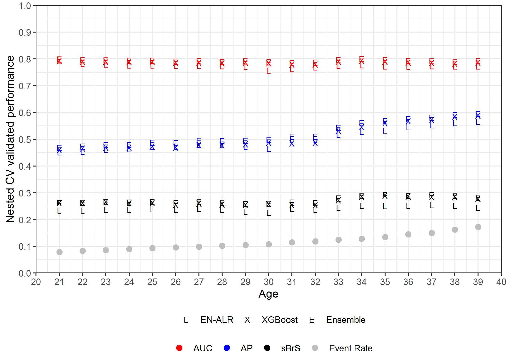
XGBoost and Ensemble provided comparable values of AUC, AP, sBrS which were always higher than that of EN-ALR regardless of age. Between XGBoost and Ensemble, Ensemble presented slightly better performance. This pattern remained the same across different ages from 21 to 39 (shown in Figure 4.3). Overall, the Ensemble algorithm achieved the best performance among the three algorithms at different ages: its AUCs were around 0.8 (ranged from 0.785 at age 31 to 0.801 at age 34), AP increased from 0.469 at age 21 to 0.595 at age 39 as event rates increased (from 0.079 at age 21 to 0.173 at age 39), and sBrS ranged from 0.259 at age 29 to 0.292 at age 37.

Figure 4.3: AUC, AP, sBrS at ages from 21 to 39
Figure 4.4 showed the calibration curves for the three algorithms at the age threshold from age 21 to 39. The calibration curves before age 28 followed the diagonal line well, indicating that the predicted risk had good alignment with the observed events. However, after age 28, the calibration curves started to deviate from the diagonal line. Serious deviations were presented after age 30, suggesting that the models were not well calibrated for ages over 30.

Figure 4.4: Calibration curves from EN-ALR, XGBoost, and Ensemble for different ages
4.4.3 Predicted risks
As the Ensemble algorithm achieved the best-validated performance, it was used to predict the risk of age-specific POI in the whole data set. It should be noted that the final predicted risks for individuals were obtained by averaging the predicted risks from the 125 work data sets.
Based on the suggestions from endocrinologists and pediatric oncologists, the predicted risks were stratified into four categories: <5%, 5% to <20%, 20% to <50%, and ≥50%, representing low, medium-low, medium, and high-risk groups, respectively. Table 4.6 (all the numbers were weighted with IPCW weights) illustrated how the Ensemble algorithm categorized survivors into four categories.
| Predicted Risk | age24:POI/Survivor | age24: POI rate | age29:POI/Survivor | age29: POI rate |
|---|---|---|---|---|
| <5% | 51/3395 | 1.5% | 11/1423 | 0.8% |
| 5% to <20% | 278/3770 | 7.4% | 370/5474 | 6.8% |
| 20% to < 50% | 147/330 | 44.5% | 139/294 | 47.2% |
| >=50% | 231/290 | 79.6% | 280/341 | 81.9% |
Specifically, at age 24, 3495 (44.9%) of 7786 participants were estimated to be at low risk (52 [1.5%] developed POI), whereas 290 (3.7%) individuals were estimated to be at high risk (231 [79.7%] developed POI). At age 29, 1423 (18.9%) of 7533 participants were estimated to be at low risk (11 [0.8%] developed POI), whereas 341 (4.5%) individuals were estimated to be at high risk (280 [82.1%] developed POI). The results suggest that the Ensemble algorithm can successfully distinguish between survivors with low-risk and high risk.
4.5 Discussion
In line with the established risk factors in the literature, the results from both EN-ALR and XGBoost showed that BMT, minimum ovarian radiation dose, cyclophosphamide dose, and procarbazine dose were associated with the risk of developing POI. EN-ALR also identified the age at diagnosis as an effect modifier of BMT which was consistent with the findings of Clark (2020)8. Besides, both algorithms identified race black and other might have a higher risk of developing POI than white, which has not been well recognized in previous research. Therefore, although the predictors were automatically selected, they can still give some insight into investigating the risk factors of developing POI. However, it should be noted that these predictors were chosen because they can improve prediction accuracy, which, however, does not imply that they cause POI. To conclude a causal relationship, a different research path is needed.
This research carefully designed the procedure of model evaluation to avoid the issue of overfitting and overoptimism. The nested CV results showed AUC could reach as high as 0.8, indicated that the models could well discriminate the subjects with POI from those without POI. The AP results were much higher than the population event rate, indicating a strong predictive power for detecting POI. The results of calibration curves showed a good alignment between predicted risks and observed events when the age threshold was less than 28, indicating that the models could well predict the probabilities of developing POI at a younger age.
The calibration results showed that long-term risk prediction can be challenging. One possible reason is that a large proportion of censoring is presented at an older age. Another reason might be that when the age threshold was farther away from the age at diagnosis, the effects of the environment or the survivors’ lifestyle may have come to play in the development of POI, which was not considered in this research.
As for the application of the final models, female survivors can be stratified into four risk categories according to estimated risks, providing useful information for them and clinicians to discuss their need for fertility preservation. Furthermore, The developed algorithm can be crafted into a user-friendly clinical tool. Appendix I presented two examples of using the tool to predict the risks of developing POI at different ages for patients.