Chapter 3 Analytical challenges and approaches

This chapter addressed challenges related to data issues including missing data and censoring. About 19% of observations had one or more missing values. Ignoring them or inappropriately dealing with them may lead to a biased inference. Section 3.1 introduced the method of multiple imputation (MI) and the procedure for conducting MI. Also, this section addressed the conflict between MI and validation methods to avoid over-optimism in the evaluation of model performance. For censoring, (i.e. some survivors with normal ovarian status did not reach the age threshold at the time they filled out the most recent survey containing MH information), section 3.2 employed the idea of inverse probability weights and highlighted how this method derived unbiased inference and dealt with the competing risk SPM.

3.1 Multiple Imputation

3.1.1 Introduction

Typically, missing data is dealt with by using the “complete-case analysis” (CCA) which ignores incomplete observations and runs analysis on the complete ones. Although this method is easy to implement and used widely in the public health field, it uses the data inefficiently because an observation will be excluded even if it has a missing value in only one variable. For example, in this project, only 6.3% of the total data was missing; however, by using CCA, almost one in five observations would be removed. Other than inefficiency, CCA may lead to biased inference when the missingness is associated with response variables. (Little and Rubin 2019; White and Carlin 2010)

To improve the inefficiency and reduce bias, MI was proposed by Rubin in 1978 (Rubin 1978) and developed in the following decades (Rubin 1996, 2004; Rubin and Schenker 1991). MI refers to the procedure of replacing each missing value with multiple imputed values,(Little and Rubin 2019) which can be thought of as drawing multiple values from the distribution of the variables given the observed data.(Little and Rubin 2019) Therefore MI returns multiple complete data sets, thus ensuring all the observed data are used to develop models. It has been theoretically proved that MI can produce valid inference in terms of unbiased parameter estimates and unbiased variance estimates under the assumption “missing at random” (MAR). MAR means missingness only depends on the observed data.(Little and Rubin 2019)

In contrast to MAR, “missing not at random” (MNAR) means that the missingness of the variable is, however, associated with the unobserved value of this variable.

Distinguishing the missingness mechanism is at the core of choosing an appropriate imputation method. However, it is impossible to differentiate MAR from MNAR based on observed data alone, because the assessment requires us to know the value of missing data.

In practice, we must use our knowledge about the study to decide whether MAR is plausible. According to the analysis in Chapter 2, we know that the missing data almost always happened in treatment variables that were abstracted from medical records. Such missingness was likely to be random when the information was collected from different hospitals rather than depending on the value of these treatments. Therefore, we can assume MAR is plausible in this study.

3.1.2 Implementation of MI

When more than one variable has missing values, we need to conduct multivariate imputation which is more challenging compared to univariate imputation. There are two general approaches for multivariate imputation: joint modeling (JM) (Schafer 1997) and fully conditional specification (FCS) (Buuren et al. 2006). While JM requires an assumption about a common prior multivariate distribution (often specified as the multivariate normal distribution) for all the variables, FCS relaxes this assumption by specifying the imputation model for each variable.

In this project, we employed the FCS approach in R package “mice” (Buuren and Groothuis-Oudshoorn 2011; Buuren and Greenacre 2018). It conducts Multivariate Imputation by Chained Equations. In this algorithm, each variable with missing data is modeled in turn conditional upon the other variables in the data. Suppose there are p variables that have missing values and M is the number of iterations, the steps of MI can be summarized as:

Step 1: Specify an imputation model for variable \(X_j\) with \(j = 1,\dots, p\);

Step 2: For each j, fill in initial imputations \(\dot{X}_j^0\) by random draws from \(X_j^{obs}\);

Step 3: Repeat for \(t = 1,\dots, M\);

Step 4: Repeat for \(j = 1,\dots, p\);

Step 5: Define \(\dot{X}_{-j}^t = \left( \dot{X}_{1}^t, \dots, \dot{X}_{j-1}^t, \dot{X}_{j+1}^t, \dots, \dot{X}_{p}^t \right)\) as the current complete data except \(X_j\);

Step 6: Build models on data \(\left(X_j^{obs} | {\dot{X}}_{-j}^t\right)\);

Step 7: Draw imputations from predicted \(X_j^{missing}\) from models built in step 6;

Step 8: End repeat \(j\);

Step 9: End repeat \(t\),

where \(X_j^{obs}\) means the observed values in \(X_j\) and \({\dot{X}}_j^t\) means imputed \(X_j\) after \(t\) th imputation.

The number of multiply imputed data sets: m

Many researchers have investigated the influence of m on different aspects of results.(Royston 2004; Graham, Olchowski, and Gilreath 2007; Bodner 2008; Von Hippel 2020; White, Royston, and Wood 2011) Basically, higher m brings benefits in terms of smaller standard errors and more replicable results. However, when the primary interest is only on point estimates, (for example, risk prediction) the high m may not be worth the time the procedure takes. In this project, we set m to be 5 considering the computation time.

3.1.3 Combining MI and nested CV

Cross-Validation (CV) is an internal validation technique, which randomly divides data set into k folds (groups) and then develops models on k–1 folds leaving out one-fold for validation. This procedure was repeated k times to utilize every fold as a validation set once. Nested CV (Varma and Simon 2006) goes one step further by constructing an inner CV in k–1 folds and utilizing the remaining fold as a test set similar to an external test set (details available in Appendix E).

An honest evaluation requires that the validation set be independent of the training set. However, the MI process uses all the observed data to predict the missing values, which “leaks” the information from the validation sets to training sets. To prevent this situation, we removed the observed values of outcome variables (menstrual status and age at event) of survivors with missing covariates in validation sets (including inner and outer validation sets in nested CV, see Appendix E) before imputation and put them back after the completion of imputation in validation sets. Figure 3.1 illustrated the procedure of combining CV and MI.

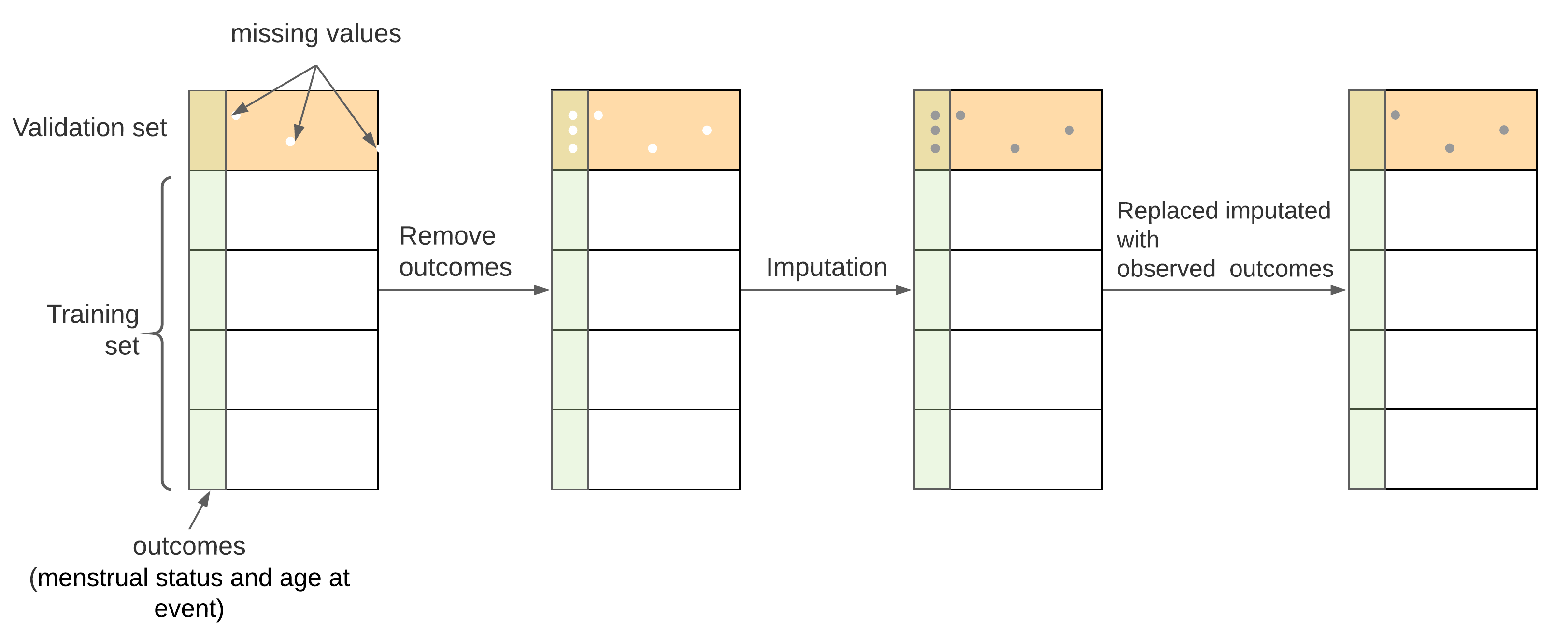
Figure 3.1: Procedure for combining MI and CV. From A to B, the outcome variables of survivors with missing covariates in validation sets were removed; from B to C, multiple imputation was conducted for both missing covariates and removed outcome variables, from C to D, original outcome variables were put back to their positions

It should be noted that every time the validation set switched, different outcome variables need to be removed accordingly, which required a new set of multiple imputations. Therefore, combining multiple imputation (\(m\)) and nested CV (\(k\)-fold outer CV and \(l\)-fold inner CV) will generate \(m \times k \times l\) complete data sets. In this study, \(m\), \(k\), and \(l\) were all set to be 5, thus there were 125 data sets generated after the MI process. They were all used for calculating IPCW and modeling the risk of POI at different ages.

3.1.4 Imputation model

In the “mice” package, various imputation methods have been built in to predict the missing values. For continuous variables, unconditional mean imputation, Bayesian linear regression, linear regression using bootstrap, etc. are available. For categorical variables, we can choose logistic regression, proportional odds models, or polytomous logistic regression. Also, predictive mean matching (PMM), classification and regression trees (CART), and random forest (RF) can be used for both continuous and categorical variables.

Among these methods, PMM avoids implausible values (e.g. negative doses) and takes heteroscedastic data into account more appropriately due to its algorithm design. PMM identifies a small subset of observations (typically up to 10) that have similar values to the predicted value for the missing entry and then drawn randomly from these candidates.(Buuren and Greenacre 2018) Besides, this procedure is much faster than another robust non-parametric algorithm RF. In this study, PMM was employed to impute all the continuous and categorical variables.

3.1.5 Convergence and the iteration number

Since the imputation was implemented using MCMC, the iteration number M should be large enough to allow the imputations to attain convergence. Appendix F assessed the convergence of imputation process. It turns out that convergence was attained when iteration number \(\geq\) 10. Therefore, the iteration M in this study was set to be 10.

3.1.6 Post-processing

In this project, age at event was missing in 38 subjects. The missing age at event relates to two ovarian status’ levels: SPM and NSPM. Based on the definition, age at NSPM should fall in the interval between (age at diagnosis + 5) and 40 (not included), and age at SPM should be between age at diagnosis and 40. To ensure the imputed ages at the event are within reasonable ranges, “post-process” functions provided in the ‘mice’ package were employed. This method only affected the synthetic values and left the observed data untouched.

The value of some variables implied the value of another variable. For example, if the dose of the irradiation to a certain body region (or a chemotherapy agent) is positive, the variable indicating patients received this irradiation (or the chemotherapy agent) should be “Yes”; otherwise, it should be “No”. For these situations, doses were imputed firstly, and the missing “Yes/No” indicators were assigned accordingly after dose imputation.

3.1.7 Results

All the missing values were successfully imputed, i.e., 5 imputation values for each missing data were generated. Because there were 25 different validation sets, a total of 125 complete data sets were obtained.

Figure 3.2 and Figure 3.3 showed the smoothed density estimation of original and imputed data for irradiation doses and chemotherapy agents’ doses, respectively. They only showed the positive doses and those with less than 20 positive doses were omitted. The imputed data and observed data had similar distributions.

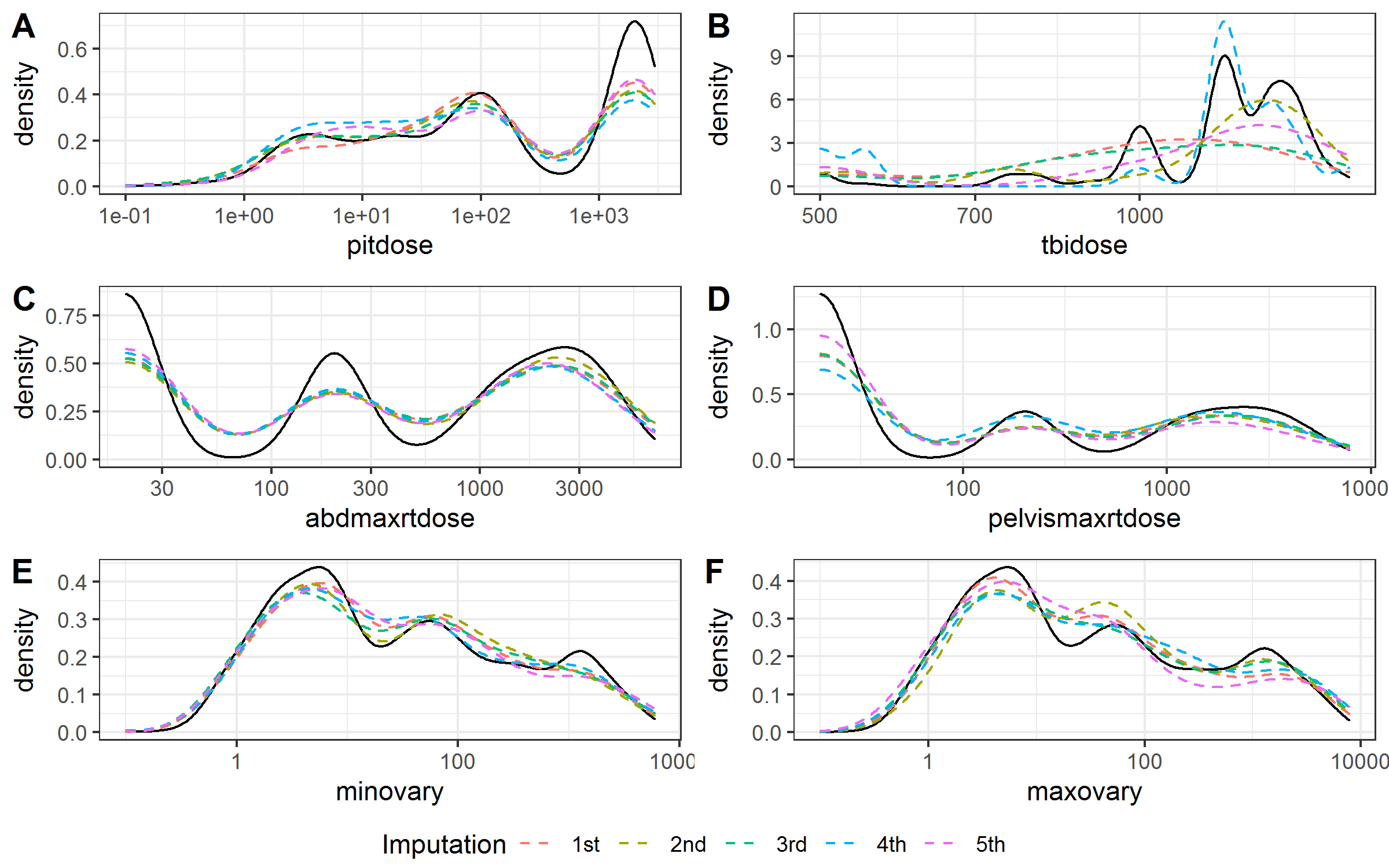
Figure 3.2: Kernel density estimates for the distributions of the radiation doses. Solid black line, observed data; dashed color lines, imputed data.

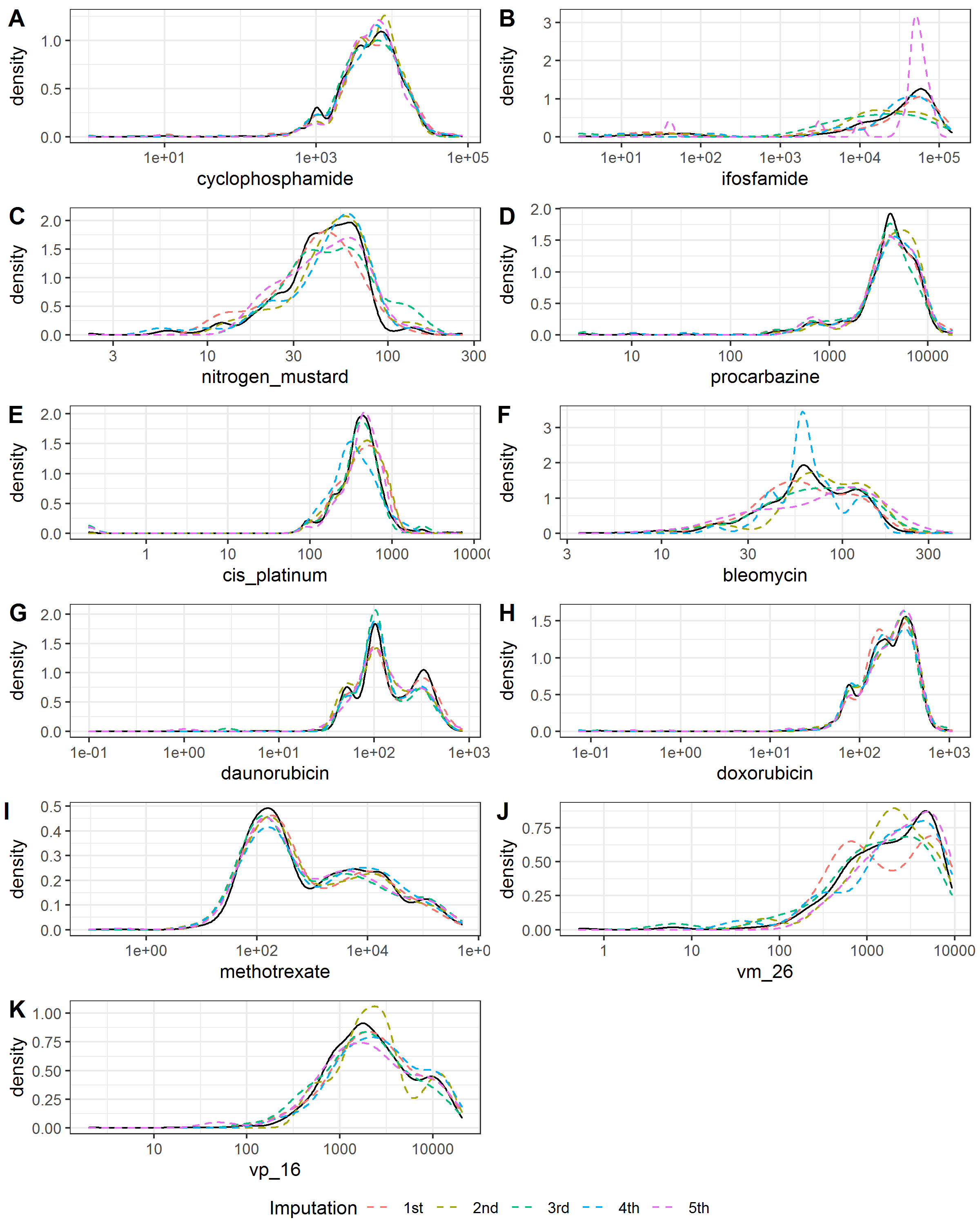
Figure 3.3: Kernel density estimates for the distributions of the chemotherapy agents’ doses. Solid black line, observed data; dashed color lines, imputed data.

Table 3.1 summarized the numbers and percentages of missing and positive values for the irradiation doses and chemotherapy agents’ doses in the observed data set and the imputed data. The imputed data had similar percentages of positive value with the observed data.

Table 3.1: Summary of frequencies and proportions of missing value and non-zero value in continuous variables.

Variable	Frequency of missing	Missing proportion	Frequency of non-zero values in observed data	Proportion of positive value in observed data	Frequency of positive values in imputed data	Proportion of non-zero value in imputed data	NA
a_event	38	0.5 %	7853	100 %	38	100 %	7891
pitdose	675	8.6 %	3469	48.1 %	319	49.9 %	7891
minovary	709	9 %	3448	48 %	363	53.9 %	7891
maxovary	715	9.1 %	3442	48 %	333	47 %	7891
tbidose	644	8.2 %	163	2.2 %	22	3.7 %	7891
abdmaxrtdose	649	8.2 %	3509	48.5 %	306	46.2 %	7891
pelvismaxrtdose	648	8.2 %	3510	48.5 %	306	48.1 %	7891
bcnu	491	6.2 %	137	1.9 %	9	3.3 %	7891
busulfan	491	6.2 %	61	0.8 %	7	1.2 %	7891
ccnu	492	6.2 %	63	0.9 %	4	1 %	7891
chlorambucil	484	6.1 %	16	0.2 %	1	0.2 %	7891
cyclophosphamide	820	10.4 %	2899	41 %	369	46.6 %	7891
ifosfamide	502	6.4 %	338	4.6 %	22	3.4 %	7891
melphalan	488	6.2 %	82	1.1 %	7	2.5 %	7891
nitrogen_mustard	530	6.7 %	324	4.4 %	32	6.6 %	7891
procarbazine	603	7.6 %	605	8.3 %	111	16.4 %	7891
thiotepa	487	6.2 %	28	0.4 %	8	2.1 %	7891
carboplatin	501	6.3 %	131	1.8 %	12	2.4 %	7891
cis_platinum	522	6.6 %	452	6.1 %	42	6.9 %	7891
bleomycin	526	6.7 %	561	7.6 %	42	9.9 %	7891
daunorubicin	543	6.9 %	1128	15.4 %	86	17.9 %	7891
doxorubicin	700	8.9 %	2654	36.9 %	288	42.6 %	7891
idarubicin	479	6.1 %	58	0.8 %	2	0.6 %	7891
methotrexate	761	9.6 %	2796	39.2 %	283	35.6 %	7891
mitoxantrone	485	6.1 %	29	0.4 %	3	0.4 %	7891
vm_26	500	6.3 %	292	4 %	27	4 %	7891
vp_16	568	7.2 %	968	13.2 %	82	15.5 %	7891

3.2 Inverse Probability Censoring Weights

3.2.1 Introduction

Censored observation is a key feature of the time to event data. The modeling of time to event data is often through accelerated failure time (AFT) models (such as Weibull, log-normal, log-logistic, etc), and semi-parametric models (Cox PH). The Cox PH model is the most popular method because it can incorporate multiple variables and does not depend on the distributional assumptions of the time variable required by the AFT models. However, Cox PH is typically used to establish the relationship between risk factors and time to event rather than to predict risk. In addition, it requires the proportional hazards assumption which may not hold in practice.(Zheng, Cai, and Feng 2006)

An alternative way to deal with the censoring problem is employing the idea of inverse probability of censoring weighting (IPCW) proposed by Robins et al in the 1990s.(Robins and Rotnitzky 1995) Using this method, we can take censoring into account by weighting observed outcomes. Then the age to event problem can be reframed to a problem with the binary outcome without losing the information of censored data, enabling the use of various classification algorithms, such as logistic regression and many popular machine learning algorithms.(Vock et al. 2016) The principle of IPCW has been well established (Zheng, Cai, and Feng 2006). The process of deriving IPCW for this study was described in the following section.

3.2.2 Derivation

The goal of this study is to estimate the probability of POI for a female childhood cancer survivor before a cut-off age \(a_0\). For a female childhood cancer survivor with covariates \(z_i\) (a realization of potential predictors \(Z\)), let random variable \(A_i\) be the POI age and random variable \(C_i\) be the censoring age.

Define the observed age at event \(X_i=min\left\{A_i,C_i\right\}\), censoring indicator \(\delta_i=I\left(A_i<C_i\right)\), and censoring status \(s_{a_0,i}\) at cut-off age \(a_0\):

\[ S_{a_{0}, i}=\left\{\begin{array}{ll} 1, & \text { if }\left(X_{i}<a_{0} \quad \& \quad \delta_{i}=1\right) \text { or }\left(X_{i} \geq a_{0}\right) \\ 0, & \text { if }\left(X_{i}<a_{0} \quad \& \quad \delta_{i}=0\right) \end{array}\right. \]

\(s_{a_0,i} = 1\) represents the ovarian status is known at age \(a_0\), \(s_{a_0,i} = 0\) represents the ovarian status is censored at age \(a_0\).

The probability of POI before \(a_0\) can be expressed as:

\[ P\left(A<a_{0} \mid Z\right)=f_{a_{0}}(Z, \theta) \]

where \(f_{a_0}\left(Z,\ \theta\right)\) is the model for estimating the probability of POI before age \(a_0\). \(\theta\) are from parameters’ space \(\mathrm{\Theta}\). For parametric models (e.g., generalized linear regression models) \(\theta\) are parameters, for non-parametric models (e.g. tree-based methods), \(\theta\) indicate how the \(Z\) space is segmented.

Solving this problem equals to finding optimal \(\theta\), and it can be obtained by solving the following minimization problem:

\[ \min _{\theta \in \Theta} \frac{1}{N} \sum_{i=1}^{N} \ell\left(f_{a_{0}}\left(z_{i}, \theta\right), y_{i}\right) \] wherein N is the number of observations, y_i is the event outcome equals to \(I\left(A_i<a_0\right)\) and \(\ell\left(\cdot\right)\) is an optimization function, for example for logistic regressions

\[ \ell\left(f_{a_{0}}\left(z_{i}, \theta\right), y_{i}\right)=y_{i} \log \left(f_{a_{0}}\left(z_{i}, \theta\right)\right)+\left(1-y_{i}\right) \log \left(1-f_{a_{0}}\left(z_{i}, \theta\right)\right) \] Due to censoring, we cannot observe all the event outcomes, and if we ignore the unobserved data, the minimization problem will become:

\[ \min _{\theta \in \Theta} \frac{1}{N} \sum_{i=1}^{N} s_{a_{0}, i} \ell\left(f_{a_{0}}\left(z_{i}, \theta\right), y_{i}\right) \]

This optimization problem leads to a misspecified \(\theta\) and a model that can not be generalized to new data. To solve this problem, we can modify the above equation using the idea of inverse probability weighting, i.e., adding the probability of remaining uncensored at \(a_0\) for each uncensored observation:

\[ \min _{\theta \in \Theta} \frac{1}{N} \sum_{i=1}^{N} \frac{s_{a_{0}, i}}{P\left(s_{a_{0}, i}\right)} \ell\left(f_{a_{0}}\left(z_{i}, \theta\right), y_{i}\right) \]

According to the definition of \(s_{a_0,i}\), \(P\left(s_{a_0,i}\right)\) can be expressed as:

\[ P\left(s_{a_{0}, i}\right)=\left\{\begin{array}{ll} P\left(C_{i}>X_{i} \mid z_{i}, A_{i}\right), & \text { if } X_{i}<a_{0}, \delta_{i}=1 \\ P\left(C_{i}>a_{0} \mid z_{i}\right), & \text { if } X_{i} \geq a_{0} \end{array}\right. \]

This modified optimization problem can give us a consistent solution for \(\theta\).

Proof:

\[ E\left\{\frac{S_{a_{0}, i}}{P\left(s_{a_{0}, i}\right)} \mid z_{i}, A_{i}\right\}=E\left\{\left[\frac{I\left(X_{i} \geq a_{0}\right)}{P\left(C_{i}>a_{0} \mid z_{i}\right)}+\frac{I\left(X_{i}<a_{0}\right) \delta_{i}}{P\left(C_{i}>X_{i} \mid Z_{i}, A_{i}\right)}\right] \mid z_{i}, A_{i}\right\}=1 \]

Here, we use the information from the entire sample to estimate \(P\left(C_i>a_0|z_i\right)\) and \(P\left(C_i>X_i|z_i,A_i\right)\). To estimate \(P\left(C_i>X_i|z_i,A_i\right)\) where A_i is not fully observed, we rely on an important assumption that the censoring process \(\mathbf{C}_\mathbf{i}\) and event process \(\mathbf{A}_\mathbf{i}\) are independent conditional on covariates \(\mathbf{z}_\mathbf{i}\). Under this assumption \(P\left(C_i>X_i|z_i,A_i\right)\) is equal to \(P\left(C_i>X_i|z_i\right)\), enabling us to use observed covariates to build an estimator \(\hat{G}\left(\cdot\right)\) for \(P\left(s_{a_0,i}\right)\). Then the estimated IPCW can be written as:

\[ \widehat{\omega}_{a_{0}, i}=\frac{S_{a_{0}, i}}{P\left(s_{a_{0}, i}\right)}=\frac{I\left(X_{i}<a_{0}\right) \delta_{i}}{\hat{G}\left(X_{i} \mid z_{i}\right)}+\frac{I\left(X_{i} \geq a_{0}\right)}{\widehat{G}\left(a_{0} \mid z_{i}\right)} \]

If the censoring process does not depend on any covariates, then \(\hat{G}\left(\cdot\right)\) can be estimated by the Kaplan-Meier method. On the other hand, if the censoring process depends on any covariates z_i, then the \(\hat{G}\left(\cdot\right)\) can be estimated by a covariate-specific survival model including Cox PH models, AFT models, and random survival forest models.

3.2.3 Competing risk

Another challenge in this study is the presence of competing risks, i.e. SPM. Once a female experienced SPM, she was not at risk of POI. Therefore, we cannot treat them as censoring. To solve this problem, we modified the IPCW formula by adding a POI indicator \(p_i\) in the first term and counting SPM as uncensoring when estimating \(\hat{G}\left(\cdot\right)\):

\[ \widehat{\omega}_{a_{0}, i}=\frac{I\left(X_{i}<a_{0}\right) I\left(p_{i}=1\right) \delta_{i}}{\widehat{G}\left(X_{i}\right)}+\frac{I\left(X_{i} \geq a_{0}\right)}{\widehat{G}\left(a_{0}\right)} \]

Therefore, in the denominator, SPM was not treated as censoring, so they did not increase the weights to the remaining survivors. On the other hand, due to the existence of POI indicator \(p_i\) in the first term, the weights for survivors with SPM ovarian status were assigned as zero, i.e., SPM did not count as an event like POI. In summary, the IPCW for different status and age at events/censoring were summarized in Table 3.2.

Table 3.2: Assignment of IPCW.

\(X_i\)	ovarian status	censoring indicator	POI indicator	\(\hat{\omega}_{a_0, i}\)
\(\leq a_0\)	Normal	0	0	0
	POI	1	1	\(1/\hat{G}(X_i)\)
	SPM	1	0	0
\(> a_0\)	Normal	0	0	\(1/\hat{G}(a_0)\)
	POI	1	0	\(1/\hat{G}(a_0)\)
	SPM	1	0	\(1/\hat{G}(a_0)\)

3.2.4 Results

Random survival forest models were fitted for estimating \(\hat{G}\left(\cdot\right)\). The variables and their importance in the survival model were presented in Figure 3.4. Age at diagnosis (“age_dx”) was the most important predictor for estimating \(\hat{G}\left(\cdot\right)\).

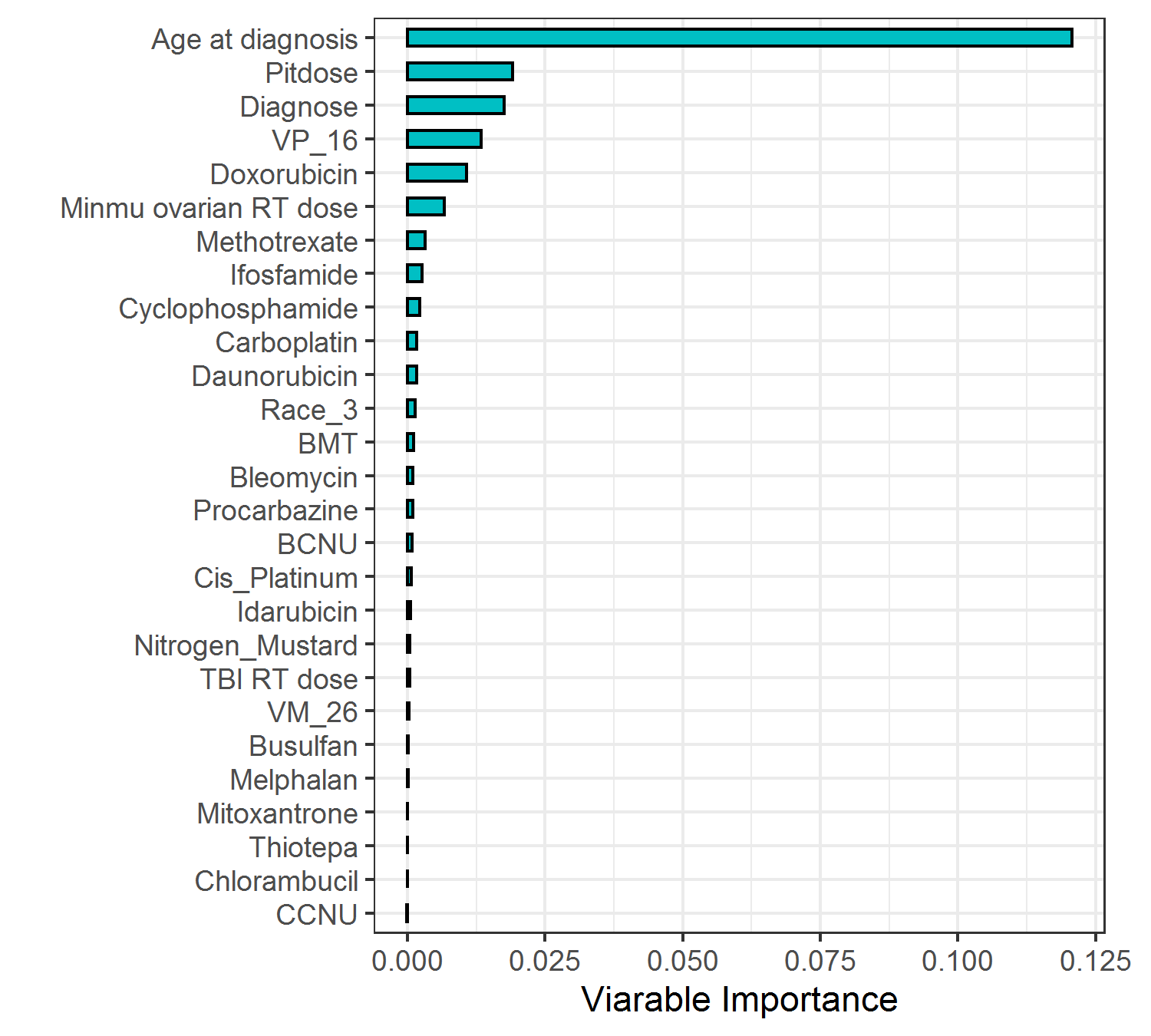
Figure 3.4: Variable importance in the random survival forest model for censoring

Figure 3.5 showed the distribution of estimated IPCW when the age threshold increased from 21 to 39. As the proportion of censoring increased with the age threshold, individuals were assigned higher IPCW and more patients were weighted to be 0 (i.e., censored). The highest IPCW was close to 30 at the largest age threshold of 39.

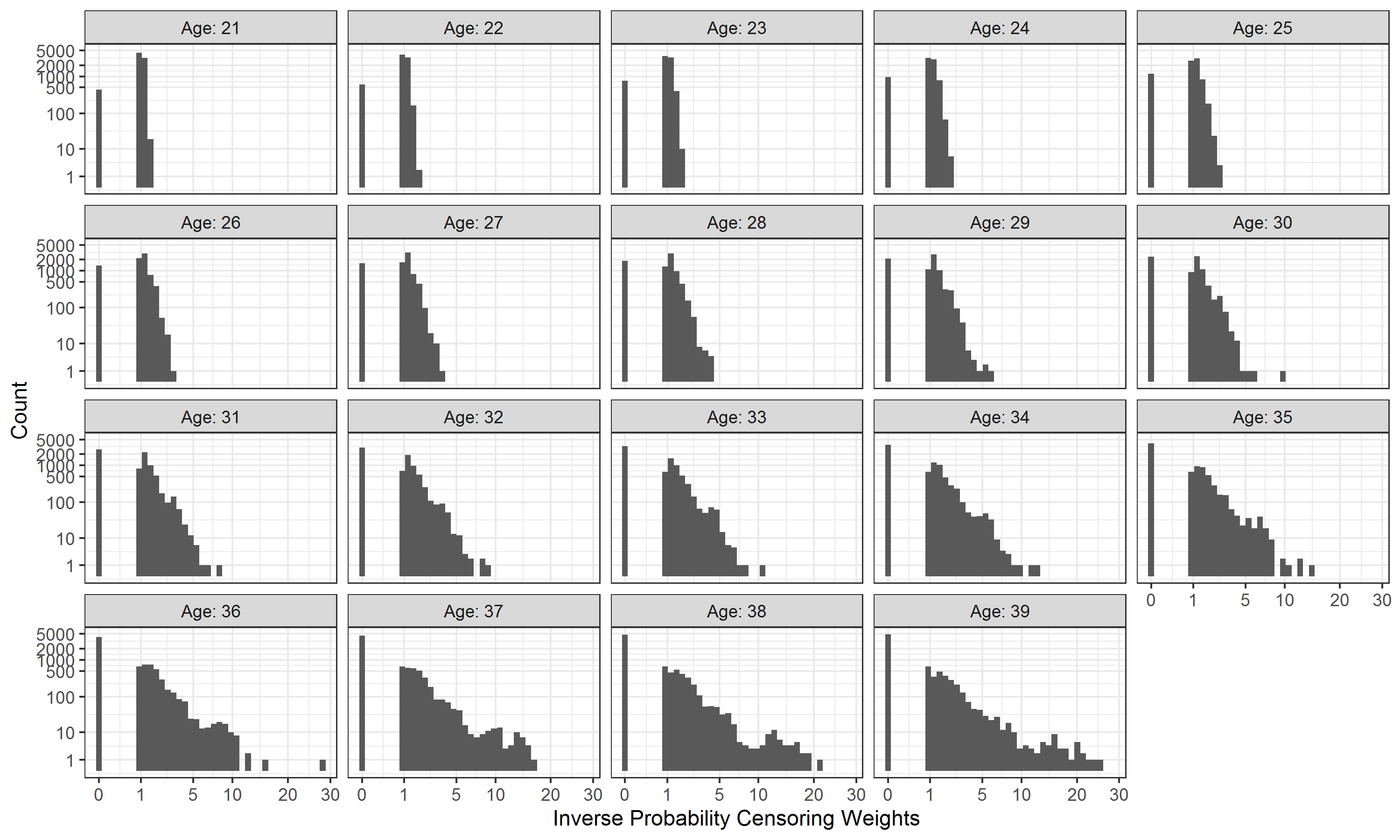
Figure 3.5: Variable importance in the random survival forest model for censoring